The notebooks folder located under your home directory contains some examples for running data manipulation, analysis and visualization.
Get started with Cartopy to produce maps and other geospatial data analyses.
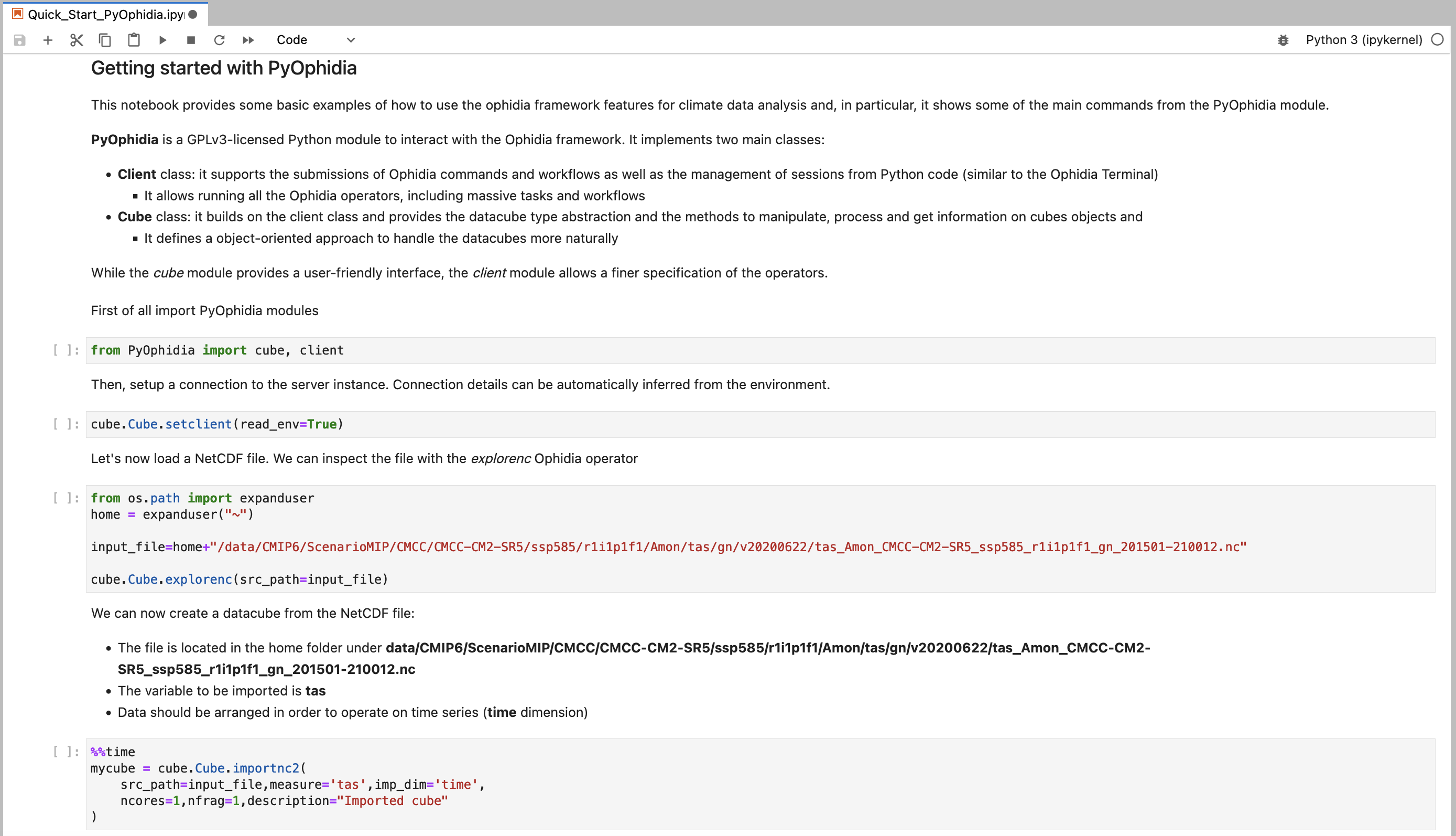
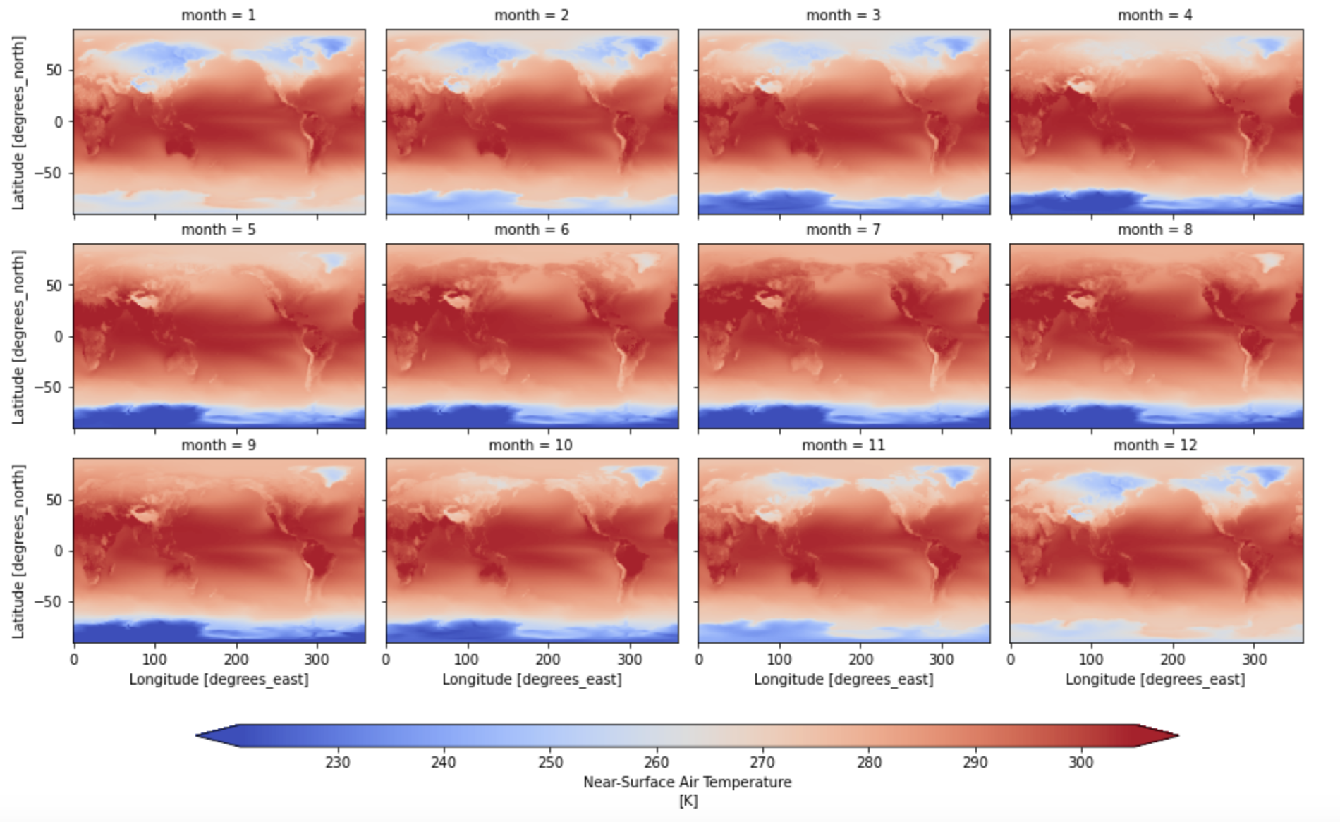
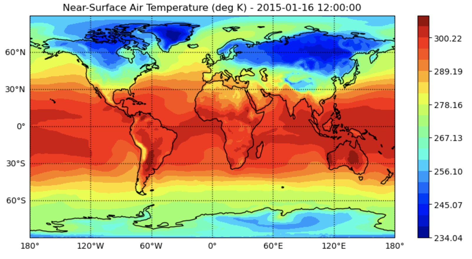
The notebook provides some basic examples of how to use the Ophidia framework features for climate data analysis through its Python bindings, PyOphidia.
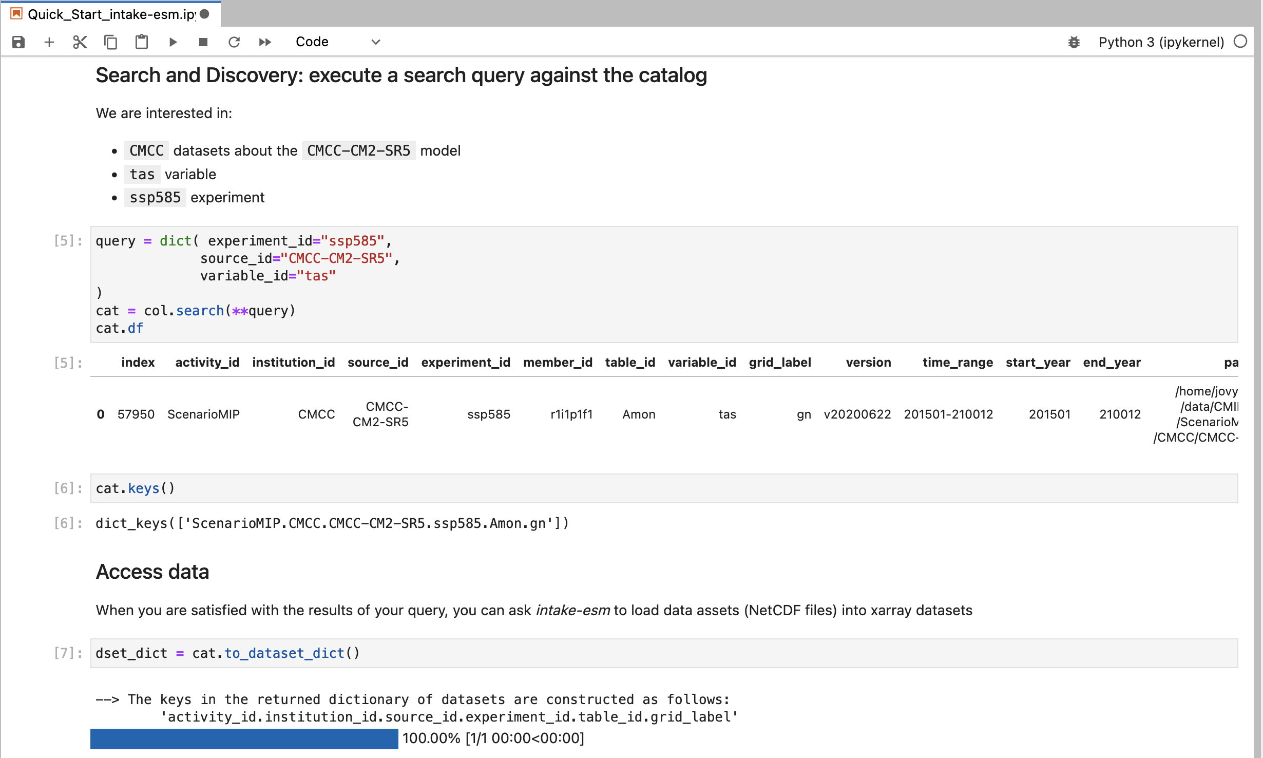
Search, discover and load CMIP6 datasets through the intake-esm data cataloging utility.
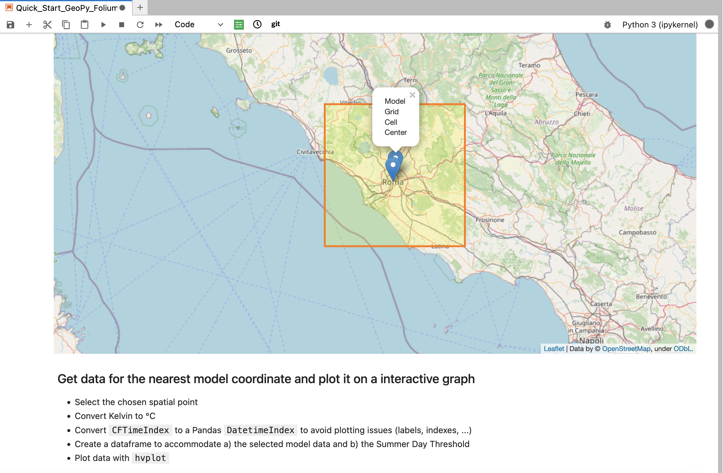
Quick Start GeoPy, Folium and hvPlot
Get started with GeoPy and Folium to deal with coordinates and interactive geographical maps, and hvplot to create interactive plots.
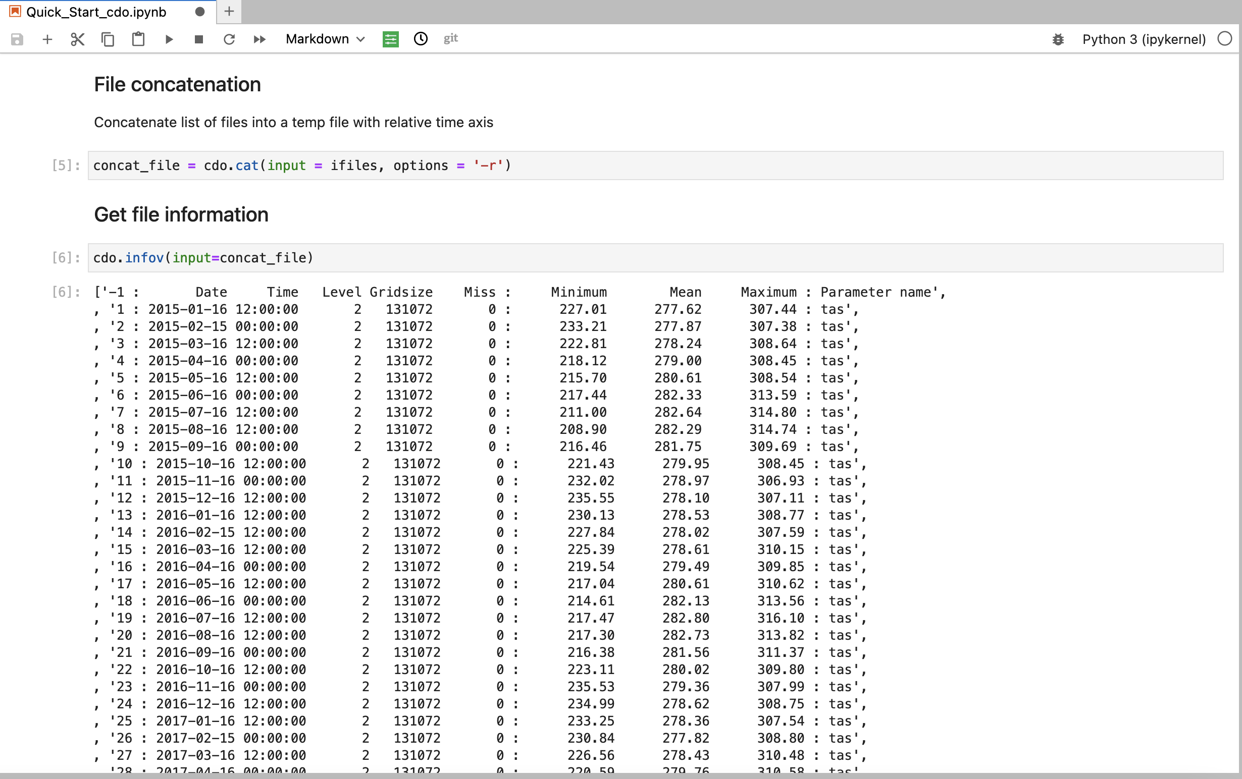
Get started with CDO (Climate Data Operators) and its Python bindings to manipulate and analyse climate model data.
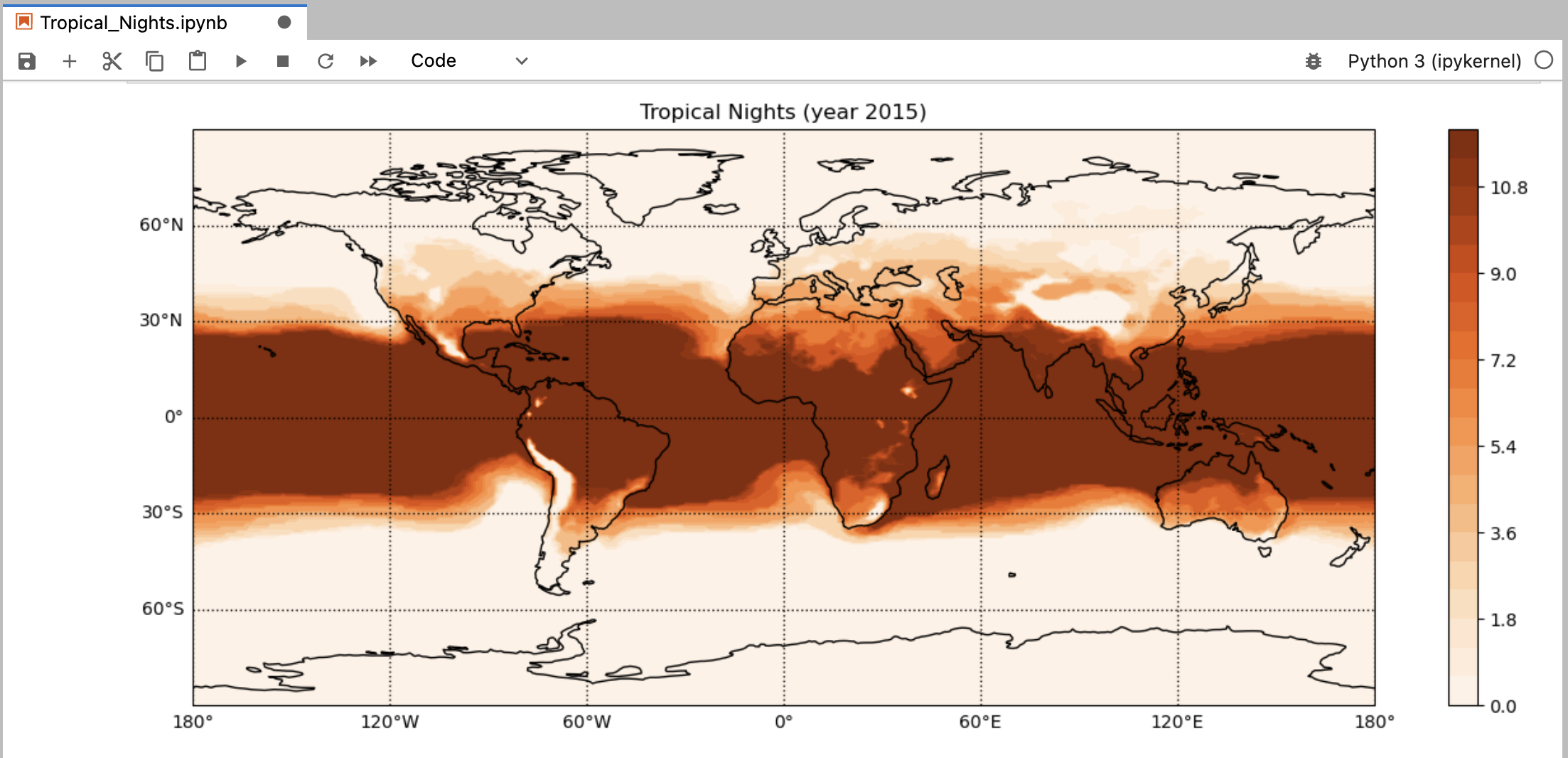
Compute the Tropical Nights Climate Index (the number of days where the daily minimum temperature is greater than 20.0C) through PyOphidia.
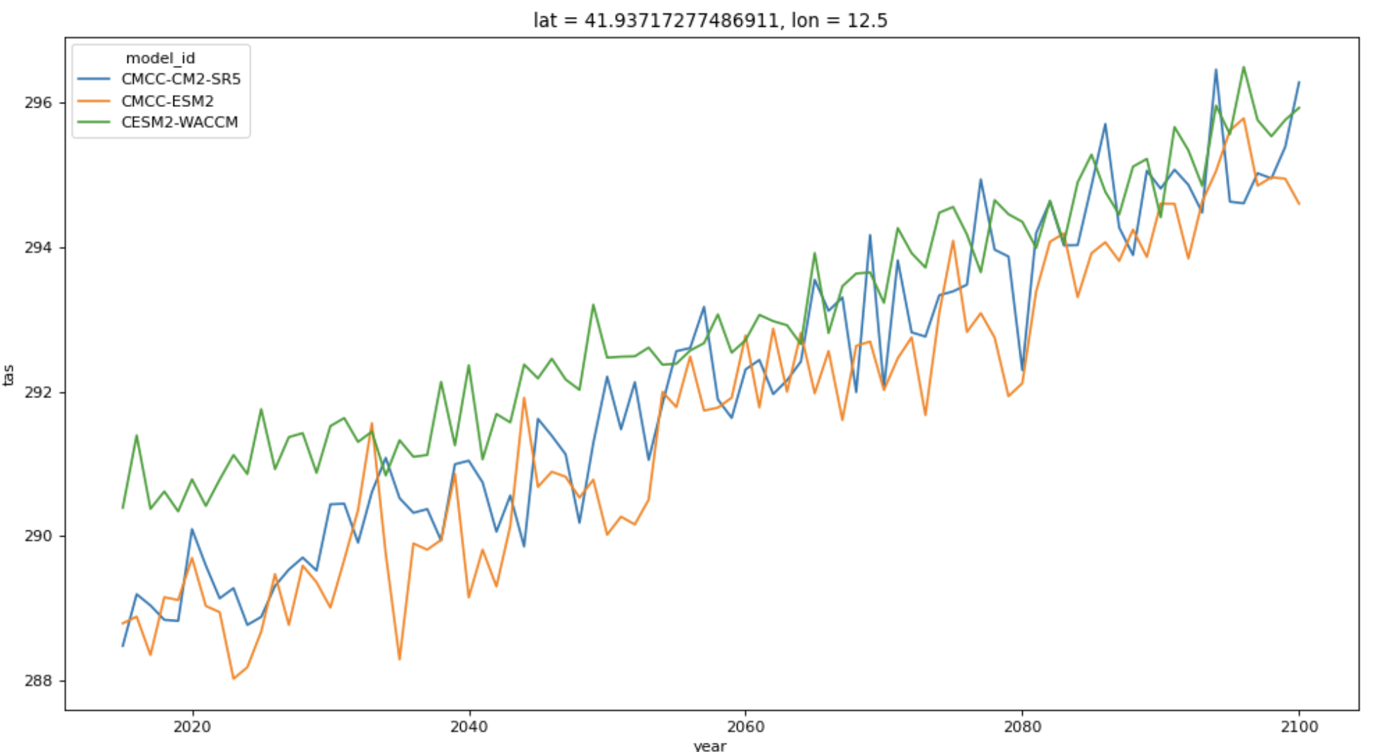
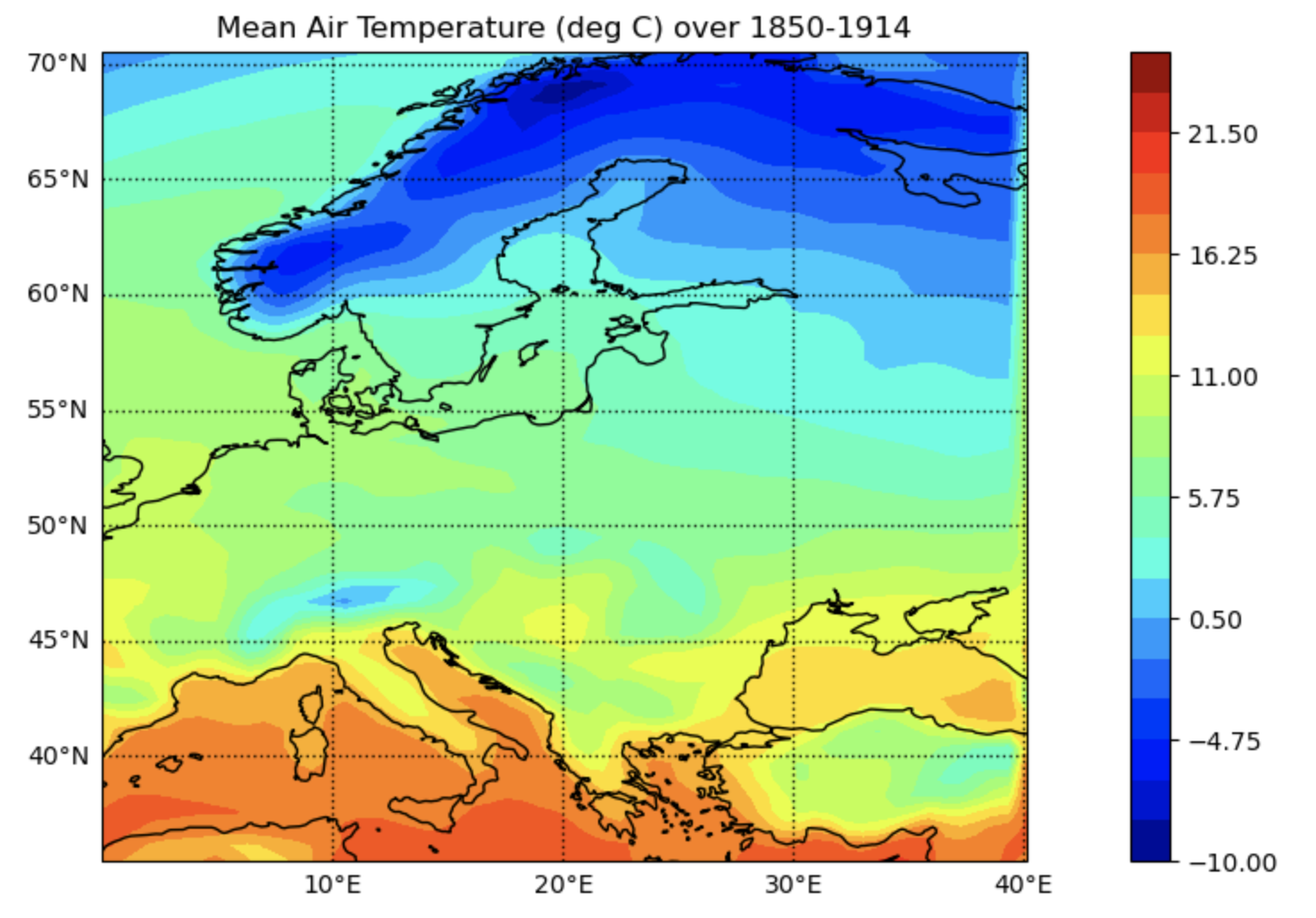
Perform a climate data analysis to compare the historical and the projected future temperature over the Europe spatial domain.
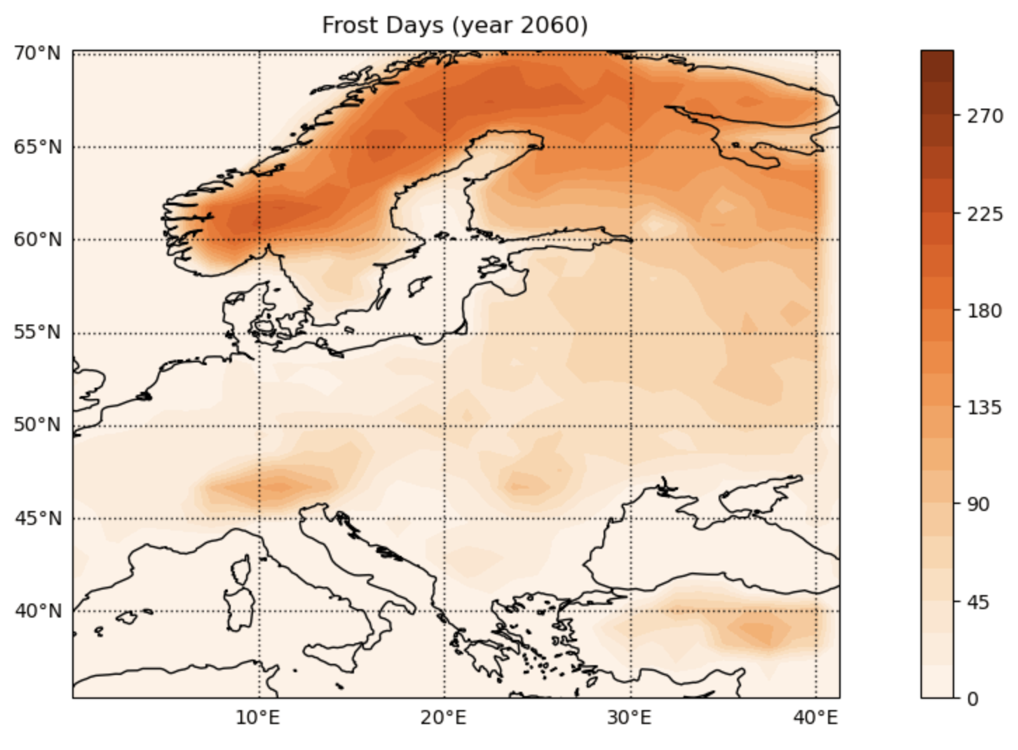
Compute the Frost Days Climate Index (the number of days where the daily minimum temperature is lower than 0C) in parallel with Dask.
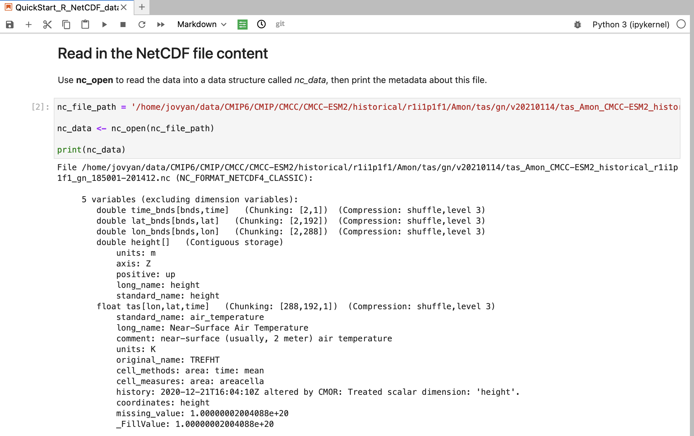
The notebook shows how to open and work with geospatial data stored in NetCDF format using the ncdf4 R package.
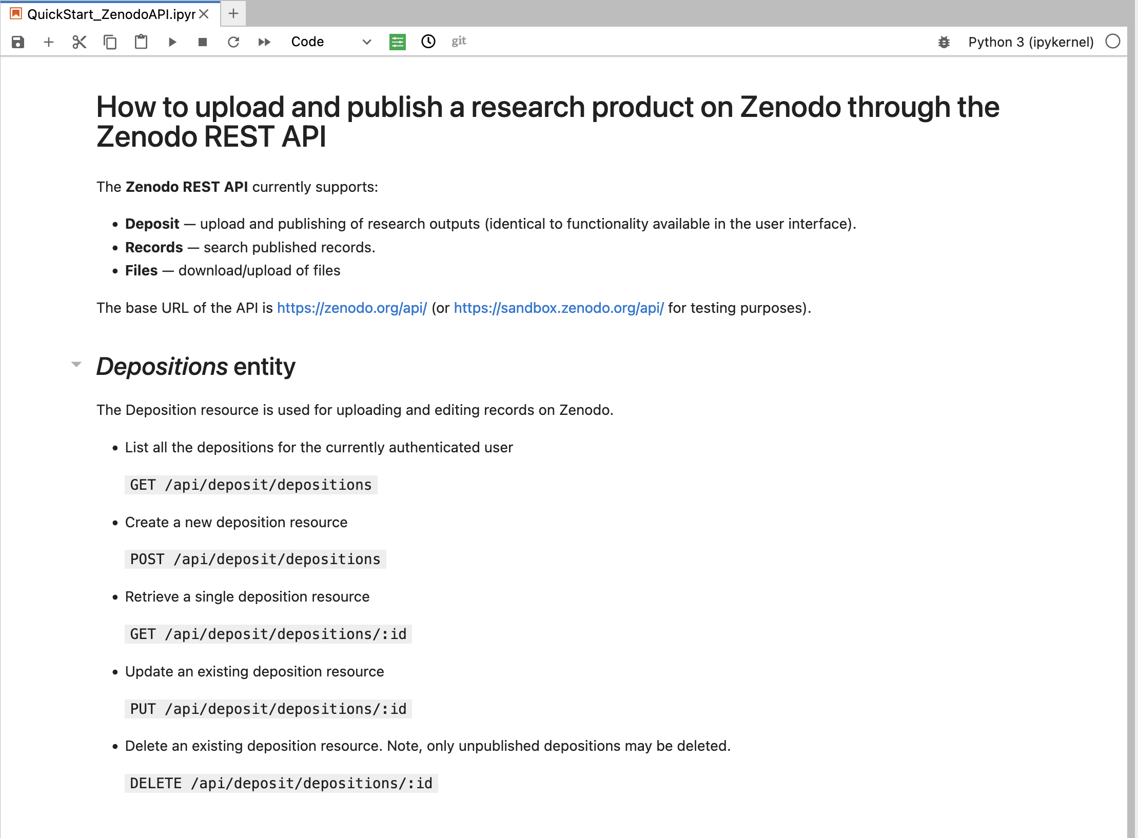
Publish a research product on Zenodo
The notebook shows how to upload and publish a research product on Zenodo through the Zenodo REST API.
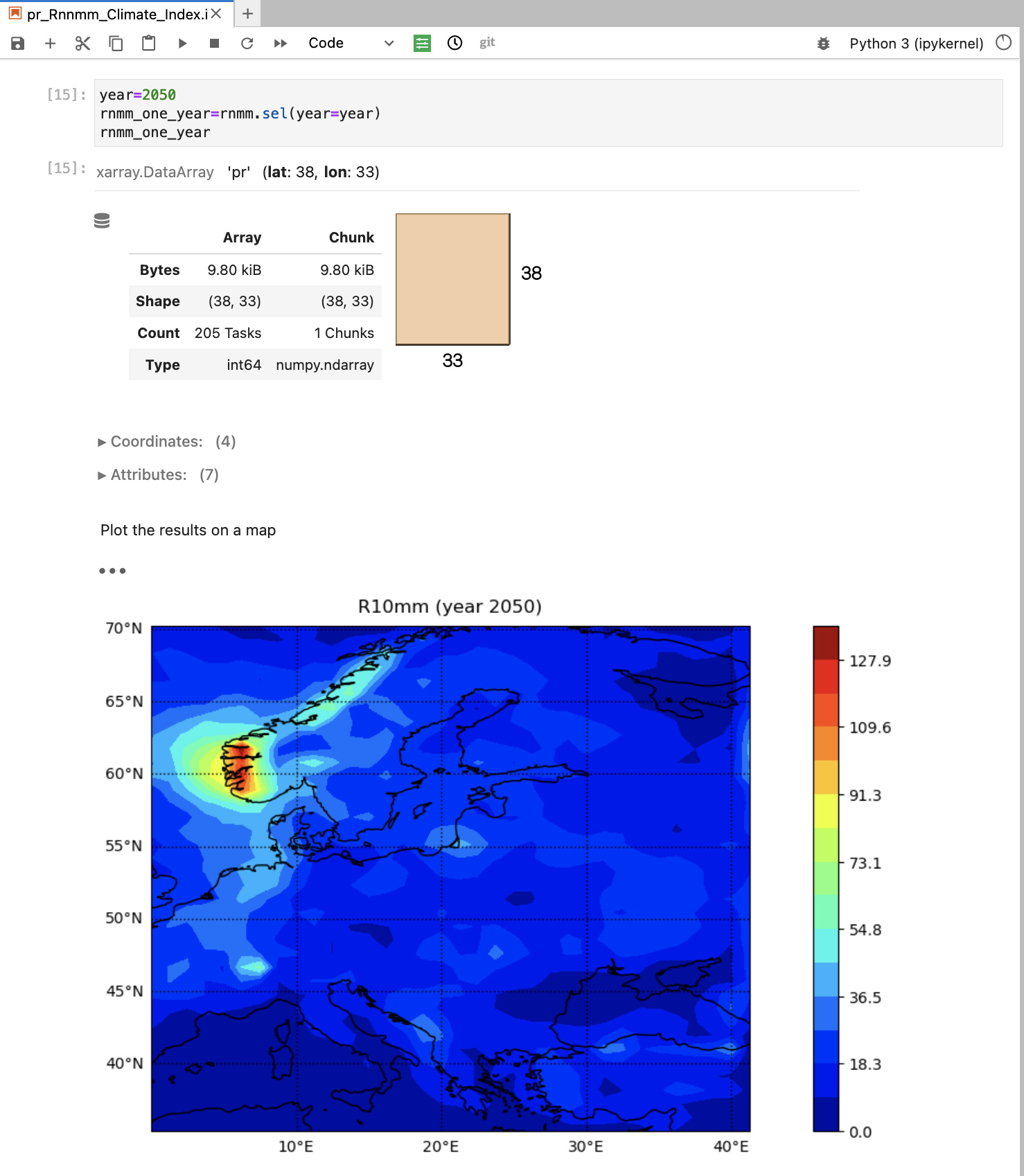
Compute the annual count of days when precipitation exceeds a given threshold (e.g., 10mm)
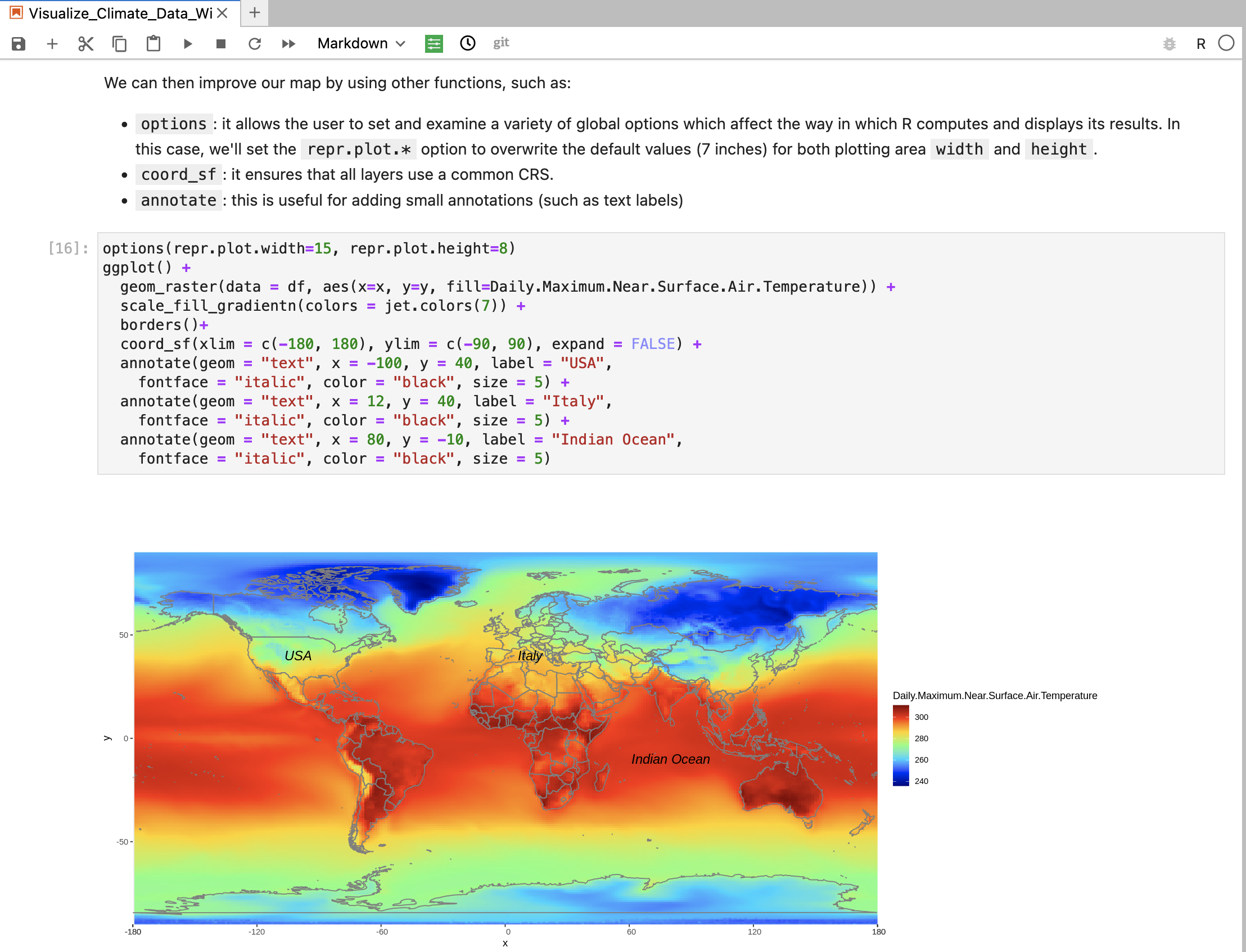
The notebook shows how to read the metadata from a NetCDF file and visualize data on a map in R.
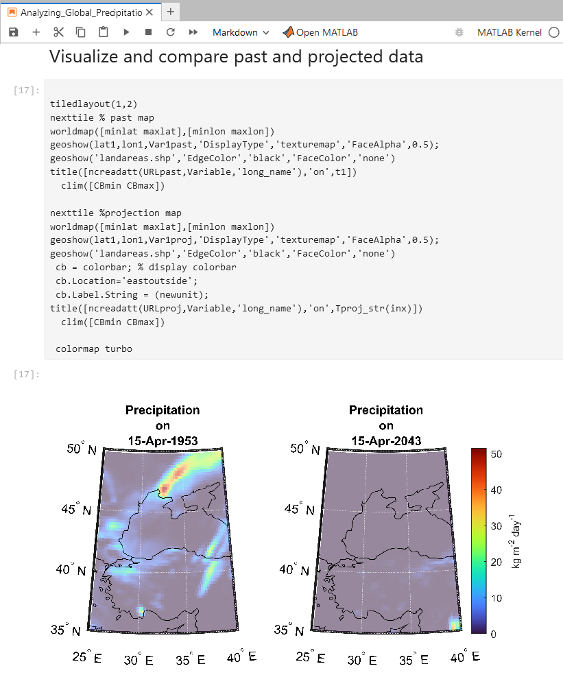
Analyze and visualize climate data with MATLAB
The notebook shows how to run MATLAB code in a Jupyter notebook using MATLAB kernel for Jupyter, or open a browser-based version of the MATLAB development environment to directly access MATLAB apps and other interactive capabilities.